For #rstats #adventofcode day 2 I decided to avoid all string parsing/manipulation/comparisons and use the command as a class to dispatch s3 methods. Is this a good idea? Probably not!
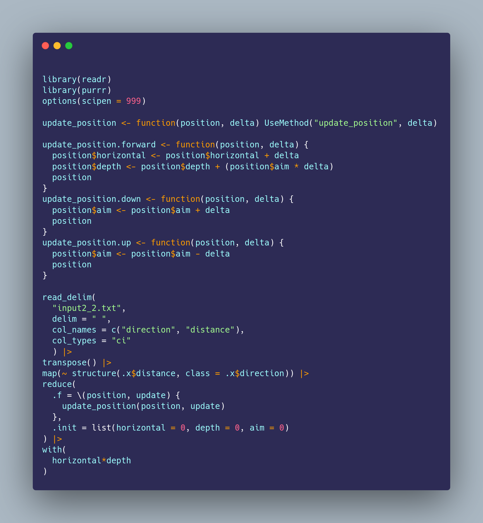
For #rstats #adventofcode day 2 I decided to avoid all string parsing/manipulation/comparisons and use the command as a class to dispatch s3 methods. Is this a good idea? Probably not!
Happy Friday #rstats {targets}/{tflow} users! Added two new addins to help smooth multi-plan workflows: Load target at cursor if found in any store in the _targets.yaml, and tar_make() the active editor plan.
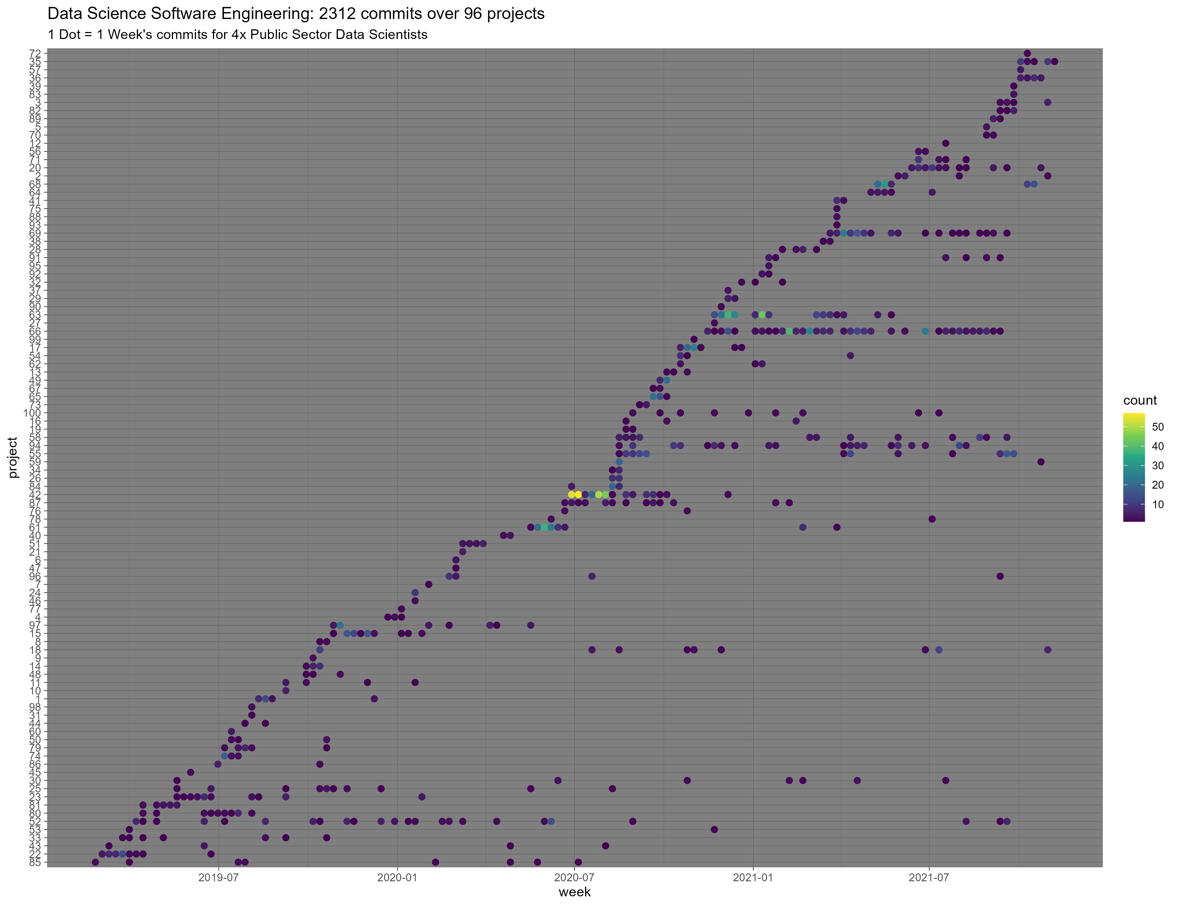
Having a second stab at a plot of my team’s commits since it has come to light that an unnamed someone was using a gmail for user.email on most of their work commits:
https://cdn.uploads.micro.blog/27894/2021/2c62b05d4a.png
I also binned the dots, instead of using alpha, and of course, that works a lot better.
Regarding software engineering for data science, I think this highlights some important issues I am going to expand on in an upcoming long-form piece. As a teaser: In a world with so many projects, and code constantly flowing between those projects, are “project-oriented workflows” that end their opinions at the project folder underfitting the needs of Data Science teams?
If you’re feeling brave I would love to compare patterns with other teams!
It’s hardly any code (if you have a flat repository structure like mine) thanks to the {gert} package:
library(gert)
library(withr)
library(tidyverse)
library(lubridate)

scan_dir <- "c:/repos"
repos <- list.dirs(scan_dir, recursive = FALSE)

all_commits <- map_dfr(repos, function(repo) {
  with_dir(repo, {
    branches <- git_branch_list() |> pluck("name")
    repo_commits <- map_dfr(branches, function(branch) {
      commits <- git_log(ref = branch)
      commits$branch <- branch
      commits
    })
    repo_commits$repo <- repo
    repo_commits
  })
})


qfes_commits <-
  all_commits |>
  filter(grepl("@qfes|North", author))


duplicates <- duplicated(qfes_commits$commit)

p <-
  qfes_commits |>
  filter(!duplicates) |>
  group_by(repo) |>
  mutate(first_commit = min(time)) |>
  mutate(repo_num = cur_group_id()) |>
  ungroup() |>
  group_by(repo_num, first_commit, week = floor_date(time, "week")) |>
  summarise(
    count = n(),
    .groups = "drop"
  ) |>
  ggplot(aes(
    x = week,
    y = fct_reorder(as.character(repo_num), first_commit),
    colour = count
  )) +
  geom_point(size = 2) +
  labs(
    title = "Data Science Software Engineering: 2312 commits over 96 projects",
    subtitle = "1 Dot = 1 Week's commits for 4x Public Sector Data Scientists",
    y = "project"
  ) +
  scale_colour_viridis_c() +
  theme_dark()

ggsave(
  "commits.png",
  p,
  device = ragg::agg_png,
  height = 10,
  width = 13
)
Often when outputting stuff to a package user, the question arises: how much effort could I be bothered to put into formatting the output? The format() function in R has some really nice stuff for this, in particular: alignment.
So today I’m outputting a list of packages to be updated:
arrow 5.0.0.2  ->  6.0.0.2
broom 0.7.7  ->  0.7.9
cachem 1.0.5  ->  1.0.6
cli 3.0.1  ->  3.1.0
crayon 1.4.1  ->  1.4.2
desc 1.3.0  ->  1.4.0
e1071 1.7-8  ->  1.7-9
future 1.22.1  ->  1.23.0
gargle 1.1.0  ->  1.2.0
generics 0.1.0  ->  0.1.1
gert 1.3.2  ->  1.4.1
googledrive 1.0.1  ->  2.0.0
googlesheets4 0.3.0  ->  1.0.0
haven 2.4.1  ->  2.4.3
htmltools 0.5.1.1  ->  0.5.2
jsonvalidate 1.1.0  ->  1.3.1
knitr 1.34  ->  1.36
lattice 0.20-44  ->  0.20-45
lubridate 1.7.10  ->  1.8.0
lwgeom 0.2-7  ->  0.2-8
mime 0.11  ->  0.12
osmdata 0.1.6.007  ->  0.1.8
paws.common 0.3.12  ->  0.3.14
pillar 1.6.3  ->  1.6.4
pkgload 1.2.1  ->  1.2.3
qfesdata 0.2.9011  ->  0.2.9030
reprex 2.0.0  ->  2.0.1
rmarkdown 2.9  ->  2.10
roxygen2 7.1.1  ->  7.1.2
RPostgres 1.3.3  ->  1.4.1
rvest 1.0.1  ->  1.0.2
sf 1.0-2  ->  1.0-3
sodium 1.1  ->  1.2.0
stringi 1.7.4  ->  1.7.5
tarchetypes 0.2.0  ->  0.3.2
targets 0.7.0.9001  ->  0.8.1
tibble 3.1.4  ->  3.1.5
tinytex 0.32  ->  0.33
travelr 0.7.5  ->  0.9.1
tzdb 0.1.2  ->  0.2.0
usethis 2.0.1  ->  2.1.3
xfun 0.24  ->  0.27
Made by this code:
  cat(
    paste(
      lockfile_deps$name,
      lockfile_deps$version_lib,
      " -> ",
      lockfile_deps$version_lock
    ),
    sep = "\n"
  )
And one thing that would make it look a bit less amateurish is alignment. I laboured over this sort of stuff years ago when I wrote {datapasta} making really hard work of it - it was the source of an infamous recurring bug. This was partly because I didn’t know that if you call format() on a character vector it automatically pads all your strings to the same length:
e.g.
  cat(
    paste(
      format(lockfile_deps$name),
      format(lockfile_deps$version_lib),
      " -> ",
      format(lockfile_deps$version_lock)
    ),
    sep = "\n"
  )
Makes the output look like:
arrow         5.0.0.2     ->  6.0.0.2
broom         0.7.7       ->  0.7.9
cachem        1.0.5       ->  1.0.6
cli           3.0.1       ->  3.1.0
crayon        1.4.1       ->  1.4.2
desc          1.3.0       ->  1.4.0
e1071         1.7-8       ->  1.7-9
future        1.22.1      ->  1.23.0
gargle        1.1.0       ->  1.2.0
generics      0.1.0       ->  0.1.1
gert          1.3.2       ->  1.4.1
googledrive   1.0.1       ->  2.0.0
googlesheets4 0.3.0       ->  1.0.0
haven         2.4.1       ->  2.4.3
htmltools     0.5.1.1     ->  0.5.2
jsonvalidate  1.1.0       ->  1.3.1
knitr         1.34        ->  1.36
lattice       0.20-44     ->  0.20-45
lubridate     1.7.10      ->  1.8.0
lwgeom        0.2-7       ->  0.2-8
mime          0.11        ->  0.12
osmdata       0.1.6.007   ->  0.1.8
paws.common   0.3.12      ->  0.3.14
pillar        1.6.3       ->  1.6.4
pkgload       1.2.1       ->  1.2.3
qfesdata      0.2.9011    ->  0.2.9030
reprex        2.0.0       ->  2.0.1
rmarkdown     2.9         ->  2.10
roxygen2      7.1.1       ->  7.1.2
RPostgres     1.3.3       ->  1.4.1
rvest         1.0.1       ->  1.0.2
sf            1.0-2       ->  1.0-3
sodium        1.1         ->  1.2.0
stringi       1.7.4       ->  1.7.5
tarchetypes   0.2.0       ->  0.3.2
targets       0.7.0.9001  ->  0.8.1
tibble        3.1.4       ->  3.1.5
tinytex       0.32        ->  0.33
travelr       0.7.5       ->  0.9.1
tzdb          0.1.2       ->  0.2.0
usethis       2.0.1       ->  2.1.3
xfun          0.24        ->  0.27
Cool hey?
A lot of the automations I rig up in my code editor depend on decting where the cursor is in a document and using that context to perform helpful operations.
The simplest class of these are functions that are executed using the symbol the cursor is “on” as input. Typically this symbol represents an object name and typical usage would be:
str() on the object to inspect ittargets::tar_load() on the object to read it from cache into the global environmentSimple things that help keep my hands on the keyboard and my head in the flow.
RStudio poses two challenges in setting these types of things up as keyboard shortcuts:
To solve 1. we can use Garrick Aden-Buie’s {shrtcts} package. To solve 2. there’s a tiny package I wrote called {atcursor}.
Suppose we desire a shortcut to call head() on the object cursor is on. This is how we could rig that up in ~/.shrtcts.R:
#' head() on cursor object
#'
#' head(symbol or selection)
#'
#' @interactive
function()  {
  target_object <- atcursor::get_word_or_selection()
  eval(parse(text = paste0("head(",target_object,")")))
}
After that we’d:
shrtcts::add_rstudio_shortcuts(){shrtcts} can also manage the keyboard bindings with an @shortcut tag but add_rstudio_shortcuts() won’t refer to it by default. See the doco if you want to do that.atcursor::get_word_or_selection() will return a symbol the cursor is “insisde” - e.g. on a column inside the span of the string. If the symbol is namespaced the namespace is also returned, e.g: “namespace::symbol”. If the user has made a selection, that is returned, regardless of cursor position.parse and then eval, sometimes I find it easier to work with expressions. So you coud do like: target_object <- as.symbol(atcursor::get_word_or_selection()) and then build an expression with bquote:eval(bquote(
some(complicated(thing(.(target_object))
))
Without getting overly metaphysical: I think these kind of shortcuts make a lot of sense to me because I view the cursor as my avatar in this world of code before me. I navigate that world almost exclusively with keys, so coding is like piloting that little avatar around. To learn about objects or manipulate them, it makes complete sense to cruise up to them and start engaging them in a dialogue of commands, the scope of which is completely unambigous, because my avatar is in the same space as those objects. In this way, my sense of ‘where I am’ in the code is not broken.
Ofcourse it does happen, I have to jump to the console world when I don’t have a binding for what I need to do, but it feels great when I don’t!
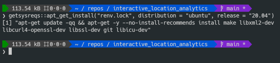
If anyone else is down for some command line JSON munging this little tool knocked my socks of this week: stedolan.github.io/jq/
Here’s a fun #rstats one from last week:
At my work, we’ve wrapped our database queries for our core datasets in an R package. Last week I needed to implement a second backend for that package such that the same interface could be used to issue fetches against either:
The idea being that pipelines that we author on our local machines should just work when running on AWS with zero changes to code. We’ll use an environment variable to control which backend our data getting functions target. So:
Sys.getenv("QFESDATA_BACKEND") == "analytics" means hit the SQL severSys.getenv("QFESDATA_BACKEND") == "aws" means slurp those parquet filesSo how to implement switching which methods are dispatched based on an environment variable? Well I definitely don’t want this:
get_oms_responses <- function() {

  if (Sys.getenv("QFESDATA_BACKEND") == "analytics") {
    ... SQL DB stuff
 } else if (Sys.getenv("QFESDATA_BACKEND") == "aws") {
   ... AWS stuff
 }
 ... common stuff
}
You CAN do that and it will work. But now the different logic for the two backends is kind of tangled together. Say I want to add a different backend in the future, I can’t do that in a way that doesn’t interact with code that is already known to work. Regressions could easily be introduced.
Isolation is what I wanted. The first thing I thought of was S3 methods, since this a bread and butter issue that S3 is designed to solve. But I thought to myself: “If I use S3 I’ll have to change the interface of my functions to refer to an object to be dispatched off.” And I didn’t like that. In other words, this type of thing:
get_oms_responses <- function(backend = "analytics", ...) UseMethod("get_oms_responses", backend)
I’d have to change all the documentation for all the functions to explain the backend arg.
So I went and implemented some complicated metaprogramming thing that detected the method you were calling and recalled a new method with the same arguments pulled from the correct parent environments based on Sys.getenv("QFESDATA_BACKEND"). I felt really smart, but the code was hard to follow, and I had to write a bunch of unit tests to convince myself it worked.
What happened next was that on seeing the code, my colleague, Anthony North, pointed out that S3 method dispatch doesn’t need to dispatch off one of the generic function arguments, it can use any object!
E.g.
get_oms_responses <- function(backend = "analytics", ...) UseMethod("get_oms_responses", ANYTHING_YOU_WANT_BUCKO)
Or perhaps more pertinently:
get_qfes_backend <- function() {
  backend <- Sys.getenv("QFESDATA_BACKEND")
  structure(backend, class = backend)
}

get_oms_responses() UseMethod("get_oms_responses", get_qfes_backend())

get_oms_responses.analytics <- function() {
  ... SQL server stuff
}

get_oms_responses.aws <- function() {
   ... AWS stuff
}
I immediately deleted what I had written and switched to this approach. Scary metaprogramming was gone, and I don’t need to unit test S3 method dispatch. It’s working perfectly.
Upon close reading of the S3 documentation, it appears this usecase is covered, barely:
for ‘UseMethod’: an object whose class will determine the method to be dispatched. Defaults to the first argument of the enclosing function.
But I’ve never seen the convenience of using any old object outside the generic function’s arguments discussed before. Quite a handy one!
Today I participated in the first meeting of the #rstats RConsortium working group for R repositories. The path I started on with cranchange lead me to this point, although this group has a much larger scope.
On the CRAN side of things I was encouraged to hear from Michael Lawrence that there is a desire to make change at CRAN including plans create a more informative public web presence, and bring on someone in a Developer Advocate role(!).
One thing I think that is going to be key to positive change is eliciting some clearer sense from CRAN as to what the group’s goals and priories are. For example: What priority is placed on being a Continuous Integration service for R-Core vs a validation and distribution mechanism for a rolling release of R packages?
I have a hunch that some of the inconsistency R users and developers see is due to tension between these types of objectives, but I am keen to learn more from this group.
I am very thankful to the Linux Foundation and RConsortium for facilitating this group, especially Joseph Rickert for leading.
Hadley Wickham’s meeting minutes are accessible from the repository
#rstats VSCode productivity tip: assign keybindings to workbench.action.terminal.scrollDown and workbench.action.terminal.scrollUp so you can move though console output without having to switch back and forth from the terminal or use your mouse.
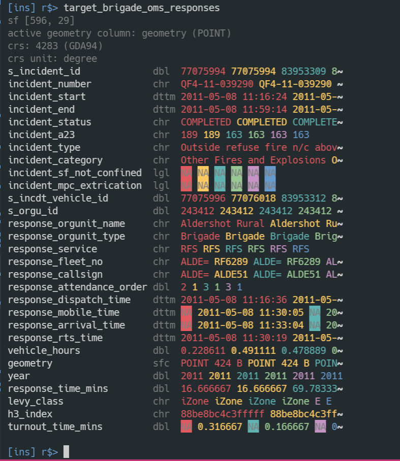
When you take advantage of {dplyr} groups for mutating or filtering you DON’T get the helpful warning about sticky groups as per summarise(). This red flag I put into {paint} has saved me twice in 2 days! #rstats
New in {rmdocs} 0.2.0:
You get an Rmd verison of the dev help for your package when it detects {devtools} is loaded. #rstats
Something in prod bombed over the weekend. I had logged the #rstats {targets} build output so I knew which target. I pulled the dependencies from the cache stepped through the target code interactively until I found the bomb. Data source schema change ofcourse. Took about ~10 minutes to pin down the field and record in the cached data and fire off the email to upsream team. Prod without a target graph and a cache? I can’t even.
In response to a Twitter question from Jared Lander, here is my logging setup:
Top level file is a .cmd - yes we’re on Windows Server Data Centre.
pushd $~dp0
Rscript.exe the_script.R > log.txt 2>&1
Roughly translated to:
Here is the_script.R:
capsule::run({
  targets::tar_invalidate(source_file)
  targets::tar_make(output)
})
Which translates to:
To do interactive diagnostics with cached targets, I run capusle::repl() to switch my R REPL over to the capsule environment.
After 7 days of dogfooding, the addition of a test suite, documentation, and 1 confirmed user, {paint} is now v0.1.0 #rstats
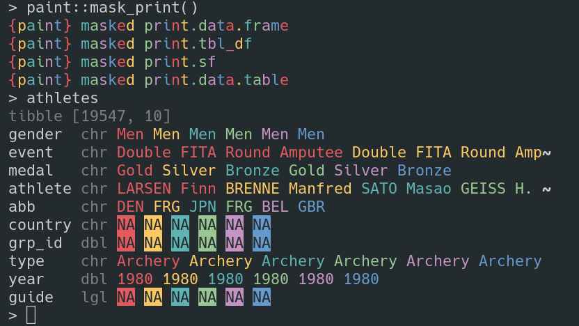
Happy Friday #rstats! This week’s diversion is alternative print() methods for data rectangles. Here’s {paint}, highly experimental, works on my machine stage:
Bit of a scraping project on that’s going to sip thousands of xml files over the next couple of days. Using #rstats {targets} dynamic branching each xml file is a cached target. The advantage of this is that if the process is interrupted at any time for any reason it can be resumed with a simple tar_make(). Niiiiiiice.
Happy Friday #rstats! Incited by @mdsumner {rmdocs} now provides replacements for utils::help and utils::?, so you never have to accidently look at HTML help again.
New {targets} addin: tflow::rs_load_current_editor_targets(). Load targets from cache that are referred to in the code you are looking at. #rstats