R is a data analysis tool, but It’s also a tool for making data analysis tools - that’s the special sauce. You take native data frames, native plotting, Lisp’s functions, and a REPL with the lot, and you can face down anything. That is why a decade in I can still find fresh ways to tackle data problems. That is why I R.

So very recently I had this situation where I had to find the needle in the haystack (It turned out to be about 20 needles, but I digress). I had to find where in thousands of lines of tidyverse-ish code, small errors were occurring that were leading to correct-ish, but progressively more incorrect results.

The code was very flat, with almost no use of functions, and a lot of repetition. Imagine something like:

data <-
  data |>
  mutate(
    intermediate_var_a = * (col2 + col3)
  )

data <-
  data |>
  mutate(
    intermediate_var_b_total = sum(intermediate_var_b),
    .by = c(group_a)
  )

data <-
  data |>
  mutate(
    scale_factor  = intermediate_var_b / intermediate_var_b_total
  )
  
data <-
  data |>
  mutate(
    `intermediate_var_c` = col5 * intermediate_var_b,
  )

data <-
  data |>
  mutate(
    intermediate_var_c = if_else(
	  intermediate_var_c < 0.00001,
	  0.00001,
	  intermediate_var_c
    ),
  )

But repeat this for thousands of lines split across about 5 files.

Maybe this style of programming feels familiar if you’ve spent a lot of time in Microsoft Excel, because that’s exactly what this was - a quite literal re-implementation of a primordial spreadsheet that had grown beyond the reasonable limits of complexity that such formats should ever contain.

In this case each row represents something quite tangible - the variables being calculated on a geographic statistical area, so that made it easy to spot areas where things had gone off the rails particularly badly by comparing variables with sources of official statistics for the area.

The question was how to put my fingers on the bugs? Checking the calculations is frustrating because they are all expressions that operate on vectors. They output reams of numbers related to hundreds of statistical areas, and the finer details get lost.

Also, many of the calculations contain interesting sub-expressions that may shed light on why things break, but you can’t interactively evaluate those though, or at least not without starting to painstakingly rewrite the code to split sub-expressions out.

I wanted an easy way to zoom in on just one row and follow that row around through the calculations. I want to pick at those sub-expressions e.g. what exactly is (1 - col1) in this case? Does that make sense? etc.

So here’s what I did. I ran the calculations through so that I had the full spectra of 300 odd columns in data. Then I used this little thing:

dive <- function(df) {
  df_env <- list2env(df)
  local(browser(), envir = df_env)
}

Then in my console:

data |>
  filter(
    id == known_broken_example
  ) |>
  dive()

So what does that do? It kicks me into a kind of ‘row-wise data debug’ mode where now every symbol in my text editor is understood to map to the corresponding row of known_broken_example. The problem has been scalarised (the reverse of vectorised maybe?).

If I highlight and run (1 - col1) I get the value that was computed for that in the context of this particular row. No need for (1 - data$col1)!

If I am cruising on down through the code I can instantly check the value of intermediate_var_c by sending it to the console etc.

I ripped through the calculations interactively, and pretty much immediately started to find threads where things didn’t seem right. It felt like I was suddenly swimming with the tide (or tidy). I could stay in my bug-hunt-flow-state without having to stop to pick apart and rewrite any code!

I’ve since added this little fella to my .Rprofile and used it in a couple of other niche cases. One more tool from the tool making machine.

This is a post I’ve been meaning to write for some time now about {capsule}.

{capsule} provides alternative workflows to {renv} for establishing and working with controlled package libraries in R. It also uses an renv.lock so it is compatible with {renv} - you can switch between doing things the {capsule} way and the {renv} or vice versa at any time.

Introducing an R package I wrote nearly three years ago

Carefully curating a controlled package environment the {renv} way can be kind of a chore. You have to init the {renv} and then be very diligent in what you install into the project library - because the project library will be “shapshotted” to create the renv.lock. {renv} provides tools to help you keep the library nice and pruned. But you have to remember to use them. And there are some challenging edge cases - particularly around ‘dev’ packages or packages that play no role in the project but aid the process of developing it.

It’s not that the {renv} way is wrong - it’s clearly not - because it’s pretty much how other languages do it, but other languages are different from R and have different developer cultures. Importantly I think R users are much more prone to interactive REPL driven development and this, in turn, lends itself to the use of interactive development tools like: {datapasta}, {ggannotate}, {esquisse} as well as other more traditional dev tools like {styler}, {lintr}. If you use VSCode you will also have packages that support the extension experience like {languageserver} and {httpgd}.

You can install these packages into the project library and by default {renv} won’t snapshot them - but then you have to go make sure your dev dependencies are up to date each time you context switch to a new project - boring! They also contaminate the project library in subtle ways: installing a new dev package might force an update of a controlled package that would have otherwise been unnecessary - should that change be reflected in the lockfile?

It all just feels a bit hard for something tangential to getting the actual work done. The hardness of keeping a clean lockfile magnifies when you have a whole team having at it with all their personal dependencies. In my case at one time we had 3 distinct text editor / IDE workflows being used within the team, not to mention each person’s preferences for RStudio addins. Some people are more onboard with putting up with some added resistance in their dev workflow than others - again the dev culture thing plays an important role as to how functional or otherwise this setup is.

Added resistance can also show up elsewhere like the time to install the local project library. And where this hurts is that this added resistance created by {renv} makes people less likely to use it. “Aww this is just an ad hoc thing, I don’t wanna jump through the hoops”. We all know by now what happens to “ad hoc things” in Data Science Land.

{capsule} provides some new lockfile workflows that are much lazier and therefore perhaps a bit easier to get adopted as standard practice for a team.

The laziest possible workflow

You’ve created a pipeline and it’s spat out the output you wanted. You didn’t use a project library to do it. You can add an renv.lock based on the project dependencies and versions in your main library with a one-liner capsule::capshot(). You commit that lockfile because one day you might need it, but you didn’t have any added resistance to your dev workflow!

In the future if you do need to run the project against the old package versions you can fire off: capsule::run(targets::tar_make()) or capsule::run(source("main.R")) or capsule::run(rmarkdown::render("report.Rmd")) etc. This will create the local project library from the lockfile and run the R command you specified against that local library. You don’t get switched into the {renv} library - so you’re not immediately flying blind without your dev tools!

Ahah but what if there’s a bug you say?! You can temporarily switch your REPL over to an R session running aginst the project library with capule::repl(). You won’t have your dev tools in this REPL though, so it may be worth doing renv::init() and going full {renv} with your dev tools installed. It’s your choice and you only pay that price if you need to.

A workflow for the whingers

Here’s a scenario that might be familiar: you have a team of people rapidly smashing out a project together. Maybe it’s a Shiny app. Someone is building the datasets, someone is wiring up the GUI, someone is making the visualisations etc. With many people contributing to an early stage project there is really no such thing as a ‘controlled package environment’.

Often issues encountered on the project force changes to internal infrastructure packages, so these are constantly updated. New packages flow into the project - particularly thanks to the GUI and vis people - they’re just going wild trying to make things look great. You all need to stay synced up with packages otherwise every time you pull changes the thing darn thing isn’t going to run.

This kind of situation is a strong argument for {renv} due to the need to stay in sync to be able run the project. However, if we slightly loosen the meaning of ‘in sync’ we can get away without the resistance of full {renv}. What I mean is: We probably don’t need to all have the exact same package versions. Over a short space of time, the culture of R developers is that packages are backward compatible with prior versions. So it’s probably fine if people are ahead of the lockfile, but less good if they fall behind.

With {capsule} we can have a workflow where we use a lockfile, but no project local library to keep us all as loosely in sync. If someone makes an important change to a package that is a dependency (or one comes down the pipe externally) we definitely need to call capsule::capshot() and commit a new lockfile. But if someone installs the latest version of {ggplot2} the day it drops because they happened not to have it, or they’re into bleeding edge - meh, we probably don’t need to update the lockfile. It’s fine for them to stay ahead of the lockfile until an important change is dropped.

What’s key is that when changes are made to the lockfile, everyone knows about them and updates the necessary packages. To do this you put capusle::whinge() somewhere in the first couple of lines of your project. It produces output like this:

> capsule::whinge()
Warning message:
In capsule::whinge() :
  [{capsule} whinge] Your R library packages are behind the lockfile. Use capsule::dev_mirror_lockfile to upgrade.

Oh but people will ignore the warning! Probably. So you can also do this, which is how my team does it:

> capsule::whinge(stop)
Error in capsule::whinge(stop) : 
  [{capsule} whinge] Your R library packages are behind the lockfile. Use capsule::dev_mirror_lockfile to upgrade.

Now it’s an error. If you’re missing any packages in the lockfile, or you’re behind the lockfile versions the project doesn’t run.

If you get this error you have a one-liner to bring yourself up to the lockfile: capsule::dev_mirror_lockfile() which will make sure you every package in your library is at least the lockfile version. Importantly packages are never downgraded. So that bleeding edge {ggplot2} person can still get those Up To Date endorphins.

I am shocked by how well this workflow works. There’s a possibility of someone using a new package version with breaking changes and forgetting to update the lockfile - and I was fully expecting this to be a big problem… but it just wasn’t. The reason I think it works is that there’s no production environment in the mix here. This is an early-stage development workflow. You’re all constantly updating and running the project, so if it breaks it gets picked up very quickly. There are only ever a few commits you need to look at to see what changed, or a quick question to your teammate who will then slap their forehead and call capsule::capshot() on their machine, commit it, and away you all go.

Finally, we’ve never felt motivated to do this, but you can tighten things up a lot with something like this:

capulse::whinge(stop)
capsule::capshot()

If all your package versions meet or exceed the lockfile, proceed immediately to creating a new lockfile, then run the project. This was actually why I created capsule::capshot(), it’s designed as a very fast ‘in-pipeline’ lockfile creator.

Conclusion

{capsule} is a package I wrote nearly 3 years ago for my team as our main R package dependency management tool. I was always hesitant to promote it because I wasn’t confident my ideas would translate well outside our team, and I also wasn’t confident I wouldn’t balls up someone’s project and they’d curse me forevermore.

It’s fairly battle-hardened now though. It has a niche little fan base of people who saw it in my {drake} post and liked it. I assume a lot of this is due to fact that there’s just less to it than {renv}. I was fairly stoked to find out it was used in the national COVID modelling pipelines in at least two countries recently. It kind of excels in that fast-paced “need something now, but can’t get all these collaborators up to speed on {renv} workflow” zone.

What I’ve learned over the last couple of years is that there isn’t ‘one workflow that fits all’ in this space. It’s about who is on the team and what that team is doing. Workflows that are standard for software engineers are sometimes hard to sell to analytic or scientific collaborators who have a different relationship with their software tool. As I have said many times in the past: If you want people to do something important, ergonomics is key! Success is much more likely with something that feels like it is “for them” rather than something that is “for someone else but we just have to live with it”. And I’m not saying I have the answer for your team, but it might be worth a look if {renv} isn’t clicking.

Finally {capsule} isn’t exactly a competitor to {renv}. It’s not fair to pitch it like that. It uses some {renv} functions under the hood. It wouldn’t have been possible if Kevin Ushey hadn’t been extremely accomodating in {renv} with some changes that enabled {capsule} to work. I think of it more as a ‘driver’ for {renv} that you can switch out at any time for the standard {renv} experience.

A lot of my work is about making tight loops.

Or maybe it’s just that as I gain mastery (slowly) of programming on datasets, the effort I expend is more around the edges of that, and the more I do that the more I understand this is a problem domain in an of itself.

For me, a tight loop is usually made by the scaffolding around the project. Typically this scaffold also made from code like the project. The scaffold’s job is to allow me to observe the effects of the project code that I write rapidly, ideally instantaneously, and to paper over context switching to keep me focussed.

The more rapidly I can get feedback the quicker I can learn if I’m on the right track and correct to eventually complete the task. While context switching and focus are intimately, and invsersely related in my experience.

In R, {targets} is a tool for making tight loops. You change a pipeline, and by the magic of caching, get to observe the effect of that change in the shorest possible time.

Likewise, {rmarkdown} is a tool for making tight loops, but focussed on scientific documents that contain assets built from code. We can change the code that builds the assets, and immediately view the resulting document, without all the slow GUI work of attaching new figures etc.

{testthat} and test suites in general are tools for rapidly collecting vast amounts of feedback about a software project. When adding new code, we can very quickly evaluate if that code has created any problems with existing functionality.

And then there’s the R REPL itself! A spectacular facilitator of tight loops for making graphics, munging data, modelling data etc. I’m supremely spoiled when I use R.

I feel the absence of these loops when they’re missing. The last project I worked on before this extended COVID break was updating a small vector tile server written in Typescript on AWS lambda. I didn’t create the project, and it was initially extremely disorienting trying to get a workflow going.

One thing I knew was that a workflow that was like: Compile to JS, zip code, upload to AWS lambda, test in browser… was not going to work for me. That feels like sludge. I could work like that, but it would cause a lot of bad feelings, and probably take even longer because I’d keep getting distracted between all the context switches.

After some research, I decided to go the “infrastructure as code” route with AWS SAM. By virtue of doing that, I got to run the lambda function locally in a simulated environment, including attaching VSCode’s debugger! That’s pretty tight. I spent probably a week setting that up before even looking into making the changes I needed to make. I think a less experienced me would have felt the pressure to just get in there and start hacking, eager to show progress. But I was able to sell the infrastructure investment to the team with the confidence that it would all be worth it once I had the tight loop rolling.

I see this need of mine cropping up in other places too: I’ve been casually working on my on bespoke keyboard design. Taking what I learned building a Corne, but realising that in a design for my unique and hand measurements.

Initially, I was physically laying out the keyboard in KiCad, and doing paper tests on a printed version. Each time I decided to move a key, I had to do a bunch of trigonometry and sometimes propagate that to many affected keys. It got quite cumbersome.

Then I discovered (well re-discovered) Ergogen (thanks Kyle Mitchell) which is a kind of parameterised framework for generating minimal ergonomic keyboard designs from configuration files. Basically AWS SAM for keyboards if you will.

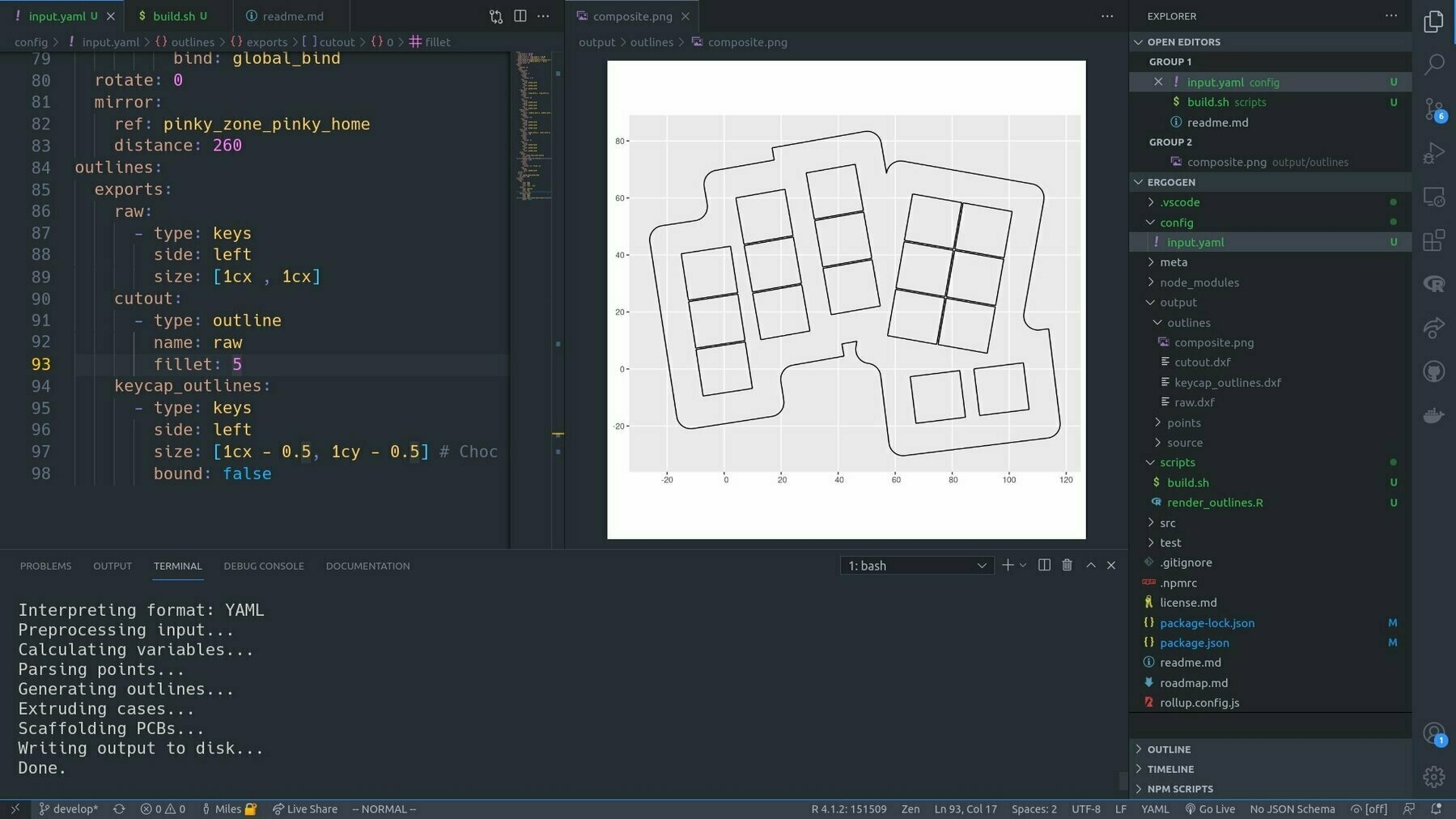
One thing I noticed was that Ergogen doesn’t ship with a quick way to do a complete visualisation of the design. But I was able to close that loop by tacking a little R script on to the build process that read in the outputs as spatial data in {sf} and plotted them with {ggplot2}.

If I have the plot image open in VSCode, it’s automatically refreshed every time I build the config. Tight loop achieved!

It’s such a powerful concept: investing in the infrastructure of the doing, to boost feedback and minimise context switching. It’s the UI for building the UI. Developer UI. Meta UI?

On reflection, I’ve been into meta UI stuff for a while now. At some level, pretty much all my open source projects are about tightening the loop: Smoothing out annoying snarls that slow down project iteration speed.

Thinking about valuing these things in this context is new for me though.

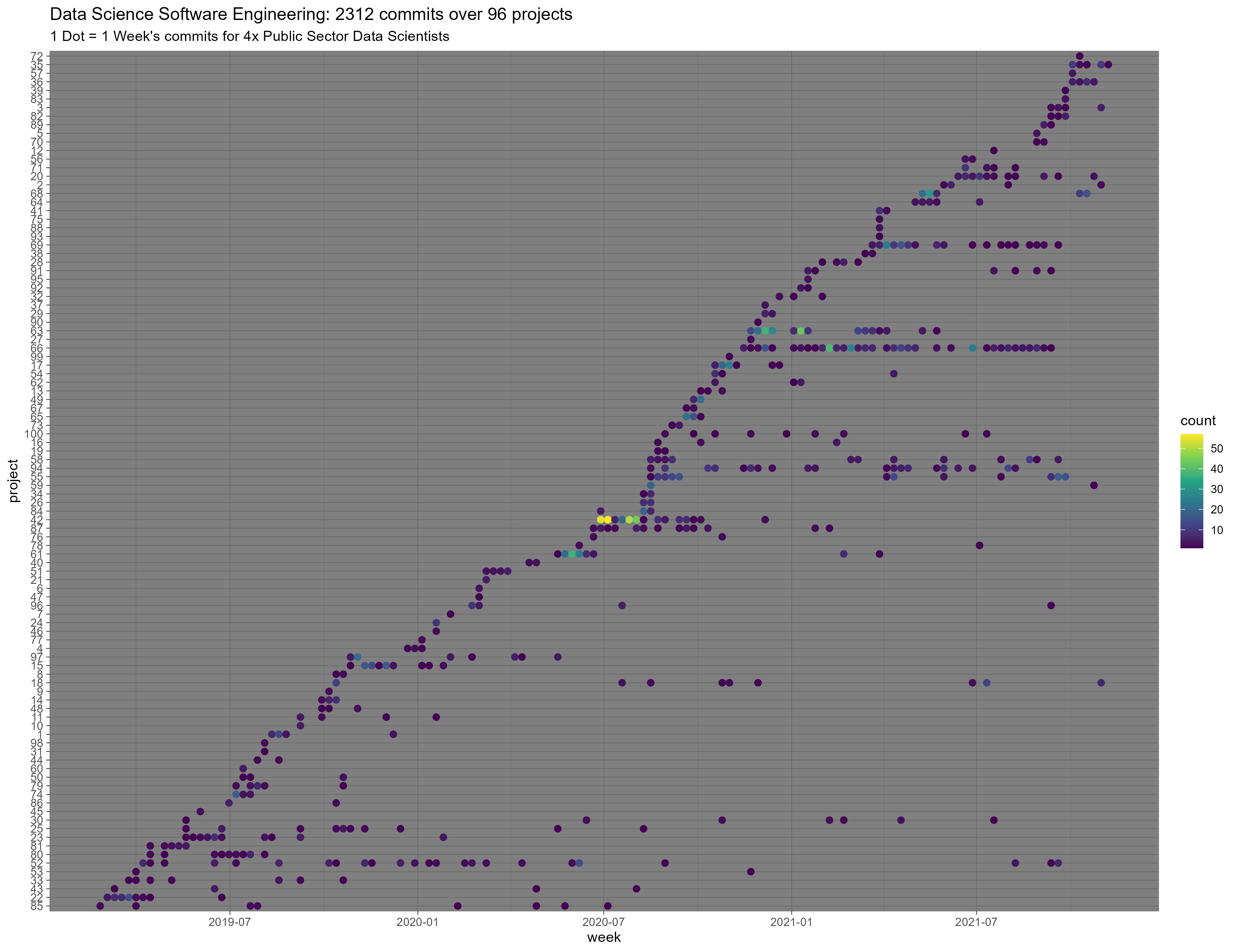
Having a second stab at a plot of my team’s commits since it has come to light that an unnamed someone was using a gmail for user.email on most of their work commits:

https://cdn.uploads.micro.blog/27894/2021/2c62b05d4a.png

I also binned the dots, instead of using alpha, and of course, that works a lot better.

Regarding software engineering for data science, I think this highlights some important issues I am going to expand on in an upcoming long-form piece. As a teaser: In a world with so many projects, and code constantly flowing between those projects, are “project-oriented workflows” that end their opinions at the project folder underfitting the needs of Data Science teams?

Make your own

If you’re feeling brave I would love to compare patterns with other teams!

It’s hardly any code (if you have a flat repository structure like mine) thanks to the {gert} package:

library(gert)
library(withr)
library(tidyverse)
library(lubridate)

scan_dir <- "c:/repos"
repos <- list.dirs(scan_dir, recursive = FALSE)

all_commits <- map_dfr(repos, function(repo) {
  with_dir(repo, {
    branches <- git_branch_list() |> pluck("name")
    repo_commits <- map_dfr(branches, function(branch) {
      commits <- git_log(ref = branch)
      commits$branch <- branch
      commits
    })
    repo_commits$repo <- repo
    repo_commits
  })
})


qfes_commits <-
  all_commits |>
  filter(grepl("@qfes|North", author))


duplicates <- duplicated(qfes_commits$commit)

p <-
  qfes_commits |>
  filter(!duplicates) |>
  group_by(repo) |>
  mutate(first_commit = min(time)) |>
  mutate(repo_num = cur_group_id()) |>
  ungroup() |>
  group_by(repo_num, first_commit, week = floor_date(time, "week")) |>
  summarise(
    count = n(),
    .groups = "drop"
  ) |>
  ggplot(aes(
    x = week,
    y = fct_reorder(as.character(repo_num), first_commit),
    colour = count
  )) +
  geom_point(size = 2) +
  labs(
    title = "Data Science Software Engineering: 2312 commits over 96 projects",
    subtitle = "1 Dot = 1 Week's commits for 4x Public Sector Data Scientists",
    y = "project"
  ) +
  scale_colour_viridis_c() +
  theme_dark()

ggsave(
  "commits.png",
  p,
  device = ragg::agg_png,
  height = 10,
  width = 13
)

Often when outputting stuff to a package user, the question arises: how much effort could I be bothered to put into formatting the output? The format() function in R has some really nice stuff for this, in particular: alignment.

So today I’m outputting a list of packages to be updated:

arrow 5.0.0.2  ->  6.0.0.2
broom 0.7.7  ->  0.7.9
cachem 1.0.5  ->  1.0.6
cli 3.0.1  ->  3.1.0
crayon 1.4.1  ->  1.4.2
desc 1.3.0  ->  1.4.0
e1071 1.7-8  ->  1.7-9
future 1.22.1  ->  1.23.0
gargle 1.1.0  ->  1.2.0
generics 0.1.0  ->  0.1.1
gert 1.3.2  ->  1.4.1
googledrive 1.0.1  ->  2.0.0
googlesheets4 0.3.0  ->  1.0.0
haven 2.4.1  ->  2.4.3
htmltools 0.5.1.1  ->  0.5.2
jsonvalidate 1.1.0  ->  1.3.1
knitr 1.34  ->  1.36
lattice 0.20-44  ->  0.20-45
lubridate 1.7.10  ->  1.8.0
lwgeom 0.2-7  ->  0.2-8
mime 0.11  ->  0.12
osmdata 0.1.6.007  ->  0.1.8
paws.common 0.3.12  ->  0.3.14
pillar 1.6.3  ->  1.6.4
pkgload 1.2.1  ->  1.2.3
qfesdata 0.2.9011  ->  0.2.9030
reprex 2.0.0  ->  2.0.1
rmarkdown 2.9  ->  2.10
roxygen2 7.1.1  ->  7.1.2
RPostgres 1.3.3  ->  1.4.1
rvest 1.0.1  ->  1.0.2
sf 1.0-2  ->  1.0-3
sodium 1.1  ->  1.2.0
stringi 1.7.4  ->  1.7.5
tarchetypes 0.2.0  ->  0.3.2
targets 0.7.0.9001  ->  0.8.1
tibble 3.1.4  ->  3.1.5
tinytex 0.32  ->  0.33
travelr 0.7.5  ->  0.9.1
tzdb 0.1.2  ->  0.2.0
usethis 2.0.1  ->  2.1.3
xfun 0.24  ->  0.27

Made by this code:

  cat(
    paste(
      lockfile_deps$name,
      lockfile_deps$version_lib,
      " -> ",
      lockfile_deps$version_lock
    ),
    sep = "\n"
  )

And one thing that would make it look a bit less amateurish is alignment. I laboured over this sort of stuff years ago when I wrote {datapasta} making really hard work of it - it was the source of an infamous recurring bug. This was partly because I didn’t know that if you call format() on a character vector it automatically pads all your strings to the same length:

e.g.

  cat(
    paste(
      format(lockfile_deps$name),
      format(lockfile_deps$version_lib),
      " -> ",
      format(lockfile_deps$version_lock)
    ),
    sep = "\n"
  )

Makes the output look like:

arrow         5.0.0.2     ->  6.0.0.2
broom         0.7.7       ->  0.7.9
cachem        1.0.5       ->  1.0.6
cli           3.0.1       ->  3.1.0   
crayon        1.4.1       ->  1.4.2
desc          1.3.0       ->  1.4.0
e1071         1.7-8       ->  1.7-9
future        1.22.1      ->  1.23.0
gargle        1.1.0       ->  1.2.0
generics      0.1.0       ->  0.1.1
gert          1.3.2       ->  1.4.1
googledrive   1.0.1       ->  2.0.0
googlesheets4 0.3.0       ->  1.0.0
haven         2.4.1       ->  2.4.3
htmltools     0.5.1.1     ->  0.5.2
jsonvalidate  1.1.0       ->  1.3.1
knitr         1.34        ->  1.36
lattice       0.20-44     ->  0.20-45
lubridate     1.7.10      ->  1.8.0
lwgeom        0.2-7       ->  0.2-8
mime          0.11        ->  0.12
osmdata       0.1.6.007   ->  0.1.8
paws.common   0.3.12      ->  0.3.14
pillar        1.6.3       ->  1.6.4
pkgload       1.2.1       ->  1.2.3
qfesdata      0.2.9011    ->  0.2.9030
reprex        2.0.0       ->  2.0.1
rmarkdown     2.9         ->  2.10
roxygen2      7.1.1       ->  7.1.2
RPostgres     1.3.3       ->  1.4.1
rvest         1.0.1       ->  1.0.2
sf            1.0-2       ->  1.0-3
sodium        1.1         ->  1.2.0
stringi       1.7.4       ->  1.7.5
tarchetypes   0.2.0       ->  0.3.2
targets       0.7.0.9001  ->  0.8.1
tibble        3.1.4       ->  3.1.5
tinytex       0.32        ->  0.33
travelr       0.7.5       ->  0.9.1
tzdb          0.1.2       ->  0.2.0   
usethis       2.0.1       ->  2.1.3
xfun          0.24        ->  0.27

Cool hey?

Here’s a fun #rstats one from last week:

At my work, we’ve wrapped our database queries for our core datasets in an R package. Last week I needed to implement a second backend for that package such that the same interface could be used to issue fetches against either:

• an on premises Microsoft SQL Server
• a set of parquet files stored in AWS S3.

The idea being that pipelines that we author on our local machines should just work when running on AWS with zero changes to code. We’ll use an environment variable to control which backend our data getting functions target. So:

• Sys.getenv("QFESDATA_BACKEND") == "analytics" means hit the SQL sever
• Sys.getenv("QFESDATA_BACKEND") == "aws" means slurp those parquet files

So how to implement switching which methods are dispatched based on an environment variable? Well I definitely don’t want this:

get_oms_responses <- function() {

  if (Sys.getenv("QFESDATA_BACKEND") == "analytics") {
    ... SQL DB stuff
 } else if (Sys.getenv("QFESDATA_BACKEND") == "aws") {
   ... AWS stuff
 }
 ... common stuff
}

You CAN do that and it will work. But now the different logic for the two backends is kind of tangled together. Say I want to add a different backend in the future, I can’t do that in a way that doesn’t interact with code that is already known to work. Regressions could easily be introduced.

Isolation is what I wanted. The first thing I thought of was S3 methods, since this a bread and butter issue that S3 is designed to solve. But I thought to myself: “If I use S3 I’ll have to change the interface of my functions to refer to an object to be dispatched off.” And I didn’t like that. In other words, this type of thing:

get_oms_responses <- function(backend = "analytics", ...) UseMethod("get_oms_responses", backend)

I’d have to change all the documentation for all the functions to explain the backend arg.

So I went and implemented some complicated metaprogramming thing that detected the method you were calling and recalled a new method with the same arguments pulled from the correct parent environments based on Sys.getenv("QFESDATA_BACKEND"). I felt really smart, but the code was hard to follow, and I had to write a bunch of unit tests to convince myself it worked.

What happened next was that on seeing the code, my colleague, Anthony North, pointed out that S3 method dispatch doesn’t need to dispatch off one of the generic function arguments, it can use any object!

E.g.

get_oms_responses <- function(backend = "analytics", ...) UseMethod("get_oms_responses", ANYTHING_YOU_WANT_BUCKO)

Or perhaps more pertinently:

get_qfes_backend <- function() { 
  backend <- Sys.getenv("QFESDATA_BACKEND")
  structure(backend, class = backend)
}

get_oms_responses() UseMethod("get_oms_responses", get_qfes_backend())

get_oms_responses.analytics <- function() {
  ... SQL server stuff
}

get_oms_responses.aws <- function() {
   ... AWS stuff
}

I immediately deleted what I had written and switched to this approach. Scary metaprogramming was gone, and I don’t need to unit test S3 method dispatch. It’s working perfectly.

Upon close reading of the S3 documentation, it appears this usecase is covered, barely:

for ‘UseMethod’: an object whose class will determine the method to be dispatched. Defaults to the first argument of the enclosing function.

But I’ve never seen the convenience of using any old object outside the generic function’s arguments discussed before. Quite a handy one!

Today I participated in the first meeting of the #rstats RConsortium working group for R repositories. The path I started on with cranchange lead me to this point, although this group has a much larger scope.

On the CRAN side of things I was encouraged to hear from Michael Lawrence that there is a desire to make change at CRAN including plans create a more informative public web presence, and bring on someone in a Developer Advocate role(!).

One thing I think that is going to be key to positive change is eliciting some clearer sense from CRAN as to what the group’s goals and priories are. For example: What priority is placed on being a Continuous Integration service for R-Core vs a validation and distribution mechanism for a rolling release of R packages?

I have a hunch that some of the inconsistency R users and developers see is due to tension between these types of objectives, but I am keen to learn more from this group.

I am very thankful to the Linux Foundation and RConsortium for facilitating this group, especially Joseph Rickert for leading.

Hadley Wickham’s meeting minutes are accessible from the repository

This week I cracked a problem that I’d been stewing on for a while: Fast generation of renv.lock files.

For those not in the know: These fully describe an R project’s package dependencies and can be used to create a “known good” package environment for the project to run in. You should definitely be using these! Typically these are created with {renv}.

I set myself a budget of 3 seconds to:

1. Detect my project dependencies
2. Read package metadata
3. Determine a full set of recursive dependencies
4. Write a lock file readable by {renv}

My thinking was that this amount of time is short enough to facilitate new workflows involving always-on automated lockfile generation. So instead of lockfile creation being a kind of manual discipline that is done interactively, it can become something that just automatically happens everytime you build a pipeline with {targets} or render a document with {rmarkdown}.

And that means people won’t forget to do it before they go on holiday, Murhpy’s law etc etc.

The generation time has to be really short because during the iteration cycle of an analysis you’re typically building a pipeline many many times in a single day. You may be adding or removing dependencies each time. Time spent waiting for things to build can rapidly become annoying, and that annoyance inspires hacks that undermine everything.

Anyway I’m happy to report success. capsule::capshot() can tick all the items I listed off in 1.5 - 2 seconds on my current project which is quite mature and laden with dependencies (~ 200 recursive deps). You give it paths to files containing your dependencies (typically a single file for me), and you get back a lockfile, built against the current .libPaths().

So you’ve likely never heard of {capsule} (although it does have its fans). It’s a kind of reimagining of the {renv} workflow for my team. It actually uses {renv} under the hood. The main point of difference is that it’s a lazy workflow. You don’t typically work out of a local library. You do that only when picking something up that’s been on the shelf for a long time, or putting something “into production” - i.e. running unsupervised somewhere.

The laziness has several advantages: You get no interaction with personal dev setups. RStudio, VSCode, Emacs, Addin packages etc… none of that needs to go anywhere near the lockfile. It’s also an easy sell. There’s 2 commands you absolutely need to know and they have obvious names: capsule::create() and capsule::run().

Some cool opportunities get opened up by the always-make-a-lockfile workflow. If we’re doing that, hopefully, we’re always committing it, and so it can become a mechanism to help nudge team-mates to keep their R libraries moving forward in step.

For example, your lockfile target could pass on building a new lockfile that would contain versions behind the current one, and send a warning to update pacakges. There’s actually machinery already in {capsule} for that, although I am still settling on the best design. I am excited to get a feel for the best practice for this kind of stuff over the next few weeks!

Due to one of my current projects, R developers have been sharing their frustrations with CRAN with me. There are many distrubing aspects to these stories, but one that is on loop in my brain at the moment is the systemic degradation CRAN policies are creating.

I think this degradation is slow and doesn’t impact too much on functionality, so it will be hard to spot at first. If there is a trend though, over time its corrosive nature will become sorely apparent. This is because developers have confessed to:

• removing all external links from documentation to avoid being flagged when one of those becomes a redirect.
• deleting examples from their code that were being run even though they were flagged with \donttest.
• suppressing tests on CRAN that were creating issues that could not be easily reproduced
• ditching vignettes that were struggling to build on CRAN

It’s kind of sad to imagine what the cumulative effect looks like of developers being nudged away from creating thoroughly tested works with rich interconnected explanatory documentation. To me, it’s just an odd situation to be in: where R itself contains excellent tools for this, but our package infrastructure is having a potentially out-sized influence on the utilisation of those tools.

Another riff on the placeholder idea with |>:

library(dplyr)
#> 
#> Attaching package: 'dplyr'
#> The following objects are masked from 'package:stats':
#> 
#>     filter, lag
#> The following objects are masked from 'package:base':
#> 
#>     intersect, setdiff, setequal, union
. <- function(.dat, template){
    template_code <- deparse(substitute(template)) 
    arg <- deparse(substitute(.dat))
    interpolated_code <- gsub("(?<=[(, ])?[.](?=[), \\[])", arg, template_code, perl = TRUE)
    eval(parse( text = interpolated_code))
}

"a" |>
 .(c(., "b")) |>
 .(setNames(., .))
#>   a   b 
#> "a" "b"

mtcars |> 
    transform(kmL = mpg / 2.35) |>
    .(lm(kmL ~ hp, data = .))
#> 
#> Call:
#> lm(formula = kmL ~ hp, data = transform(mtcars, kmL = mpg/2.35))
#> 
#> Coefficients:
#> (Intercept)           hp  
#>    12.80803     -0.02903

"col_name" |> 
  .(mutate(mtcars, . = "cool")) |>
  .(bind_cols(., .)) |>
  .(.[1, ])
#> New names:
#> * mpg -> mpg...1
#> * cyl -> cyl...2
#> * disp -> disp...3
#> * hp -> hp...4
#> * drat -> drat...5
#> * ...
#>           mpg...1 cyl...2 disp...3 hp...4 drat...5 wt...6 qsec...7 vs...8
#> Mazda RX4      21       6      160    110      3.9   2.62    16.46      0
#>           am...9 gear...10 carb...11 col_name...12 mpg...13 cyl...14 disp...15
#> Mazda RX4      1         4         4          cool       21        6       160
#>           hp...16 drat...17 wt...18 qsec...19 vs...20 am...21 gear...22
#> Mazda RX4     110       3.9    2.62     16.46       0       1         4
#>           carb...23 col_name...24
#> Mazda RX4         4          cool

^{Created on 2021-06-24 by the reprex package (v2.0.0)}

I call . the ‘neutering’ function.